Demonstration: Gradient-based optimization

In mathematics, optimization (minimization or maximization of a function) is important foundation applied for many fields such as information science, economics, bioinformatics, and physics. It is difficult to analytically solve optimization problem because a target function is very complex in practical cases. We often rely on numerical or approximation method to obtain a good solution in such cases. In this article, we introduce practical gradient-based approaches (Steepest descent, Newton method, and Quasi-Newton method) for optimization problems and how to implement them by Sized Linear Algebra Package (SLAP). You can implement the methods as easy as other linear algebra libraries.

In this article, we consider minimization problem defined as

$y = \min_{\bm{x}\in\R^n} f(\bm{x})$

where $f : \R^n\to\R$ is a target function. Minimization problem can be converted into maximization problem by replacing $f(\bm{x})$ with $-f(\bm{x})$. A target function can be non-convex, but must be differentiable. We compute a minimal point instead of an exact minimum point of a target function since the latter is hard. Gradient-based approaches use the gradient of a target function for minimization:

$\bm{\nabla}f = \left(\frac{\partial f}{\partial x_1},\dots,\frac{\partial f}{\partial x_n}\right)^\top.$

Thus we need to compute $\hat{\bm{x}}$ such that $\bm{\nabla} f(\hat{\bm{x}}) = \bm{0}$.

Preliminary

First, load SLAP on OCaml REPL or utop (# at the head of each line is prompt):

# #use "topfind";;
# #require "slap";;
# #require "slap.top";;
# #require "slap.ppx";;
# open Format;;
# open Slap.D;;
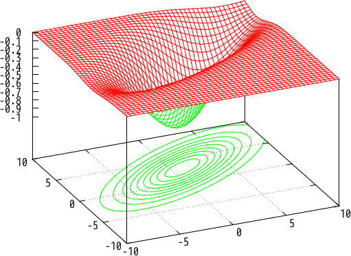
# open Slap.Io;;

Second, define target function $f$ you want to minimize. In this article, we choose a Gaussian function as a target:

$f(\bm{x})=-\exp\left(\frac{1}{2}(\bm{x}-\bm{b})^\top\bm{A}(\bm{x}-\bm{b})\right)$

where

$\bm{A}=\begin{pmatrix} -0.1&0.1\\0.1&-0.2\\ \end{pmatrix},\quad \bm{b}=(1.0,3.0)^\top.$

Note that $\bm{A}$ is symmetric, and the minimum is -1 at (1, 3).

The target is a Gaussian function — Fig 1. The target function in this demonstration

The Gaussian function is implemented as follows:

# let gauss a b x =
    let xb = Vec.sub x b in
    ~-. (exp (dot xb (symv a xb) /. 2.0));;
val gauss : ('a, 'a, 'b) mat -> ('a, 'c) vec -> ('a, 'd) vec -> float = <fun>

where dot is a Level-1 BLAS function and symv is a Level-2 BLAS function. The type of gauss means

the first argument is 'a-by-'a matrix,
the second argument is 'a-dimensional vector,
the third argument is 'a-dimensional vector, and
the return value has type float.

You can execute gauss by passing $\bm{A}$, $\bm{b}$ and $\bm{x}$:

# let a = [%mat [-0.1, 0.1;
                 0.1, -0.2]];;
val a : (Slap.Size.two, Slap.Size.two, 'a) mat =
       C1   C2
  R1 -0.1  0.1
  R2  0.1 -0.2

# let b = [%vec [1.0; 3.0]];;
val b : (Slap.Size.two, 'a) vec = R1 R2
                                   1  3

# gauss a b [%vec [0.0; 0.0]];;
- : float = -0.522045776761015934

However you cannot give vectors and matrices that have sizes inconsistent with the type of gauss as follows:

gauss a b [%vec [0.0; 0.0; 0.0]];;
Error: This expression has type
         (Slap.Size.three, 'a) vec =
           (Slap.Size.three, float, rprec, 'a) Slap_vec.t
       but an expression was expected of type
         (Slap.Size.two, 'b) vec =
           (Slap.Size.two, float, rprec, 'b) Slap_vec.t
       Type Slap.Size.three = Slap_size.z Slap_size.s Slap_size.s Slap_size.s
       is not compatible with type
         Slap.Size.two = Slap_size.z Slap_size.s Slap_size.s
       Type Slap_size.z Slap_size.s is not compatible with type Slap_size.z

The static size checking of SLAP protects you against dimensional inconsistency. If you get an error message like the above output, your program possibly has a bug.

Steepest descent method

Sample program: examples/optimization/steepest_descent.ml

Steepest descent (a.k.a., gradient descent) is a kind of iterative methods: we choose an initial value $\bm{x}^{(0)}$, and generate points $\bm{x}^{(1)},\bm{x}^{(2)},\bm{x}^{(3)},\dots$ by

$\bm{x}^{(t+1)} = \bm{x}^{(t)} - \eta \bm{\nabla}f(\bm{x}^{(t)})$

where $\eta$ is a learning rate (a parameter for controlling convergence). The above update formula is easily implemented as follows:

# let steepest_descent ~loops ~eta df f x =
    for i = 1 to loops do
      axpy ~alpha:(~-. eta) (df x) x; (* Steepest descent: x := x - eta * (df x) *)
      printf "Loop %d: f = %g, x = @[%a@]@." i (f x) pp_rfvec x
    done

Above code uses Level-1 BLAS function axpy.

The gradient of the target function is given by

$\begin{align*} \bm{\nabla}f(\bm{x}) &=-\exp\left(\frac{1}{2}(\bm{x}-\bm{b})^\top\bm{A}(\bm{x}-\bm{b})\right) \frac{1}{2}(\bm{A}+\bm{A}^\top)(\bm{x}-\bm{b})\\ &=-\exp\left(\frac{1}{2}(\bm{x}-\bm{b})^\top\bm{A}(\bm{x}-\bm{b})\right) \bm{A}(\bm{x}-\bm{b}). \end{align*}$

# let dgauss a b x = symv ~alpha:(gauss a b x) a (Vec.sub x b);;
val dgauss : ('a, 'a, 'b) mat -> ('a, 'c) vec -> ('a, 'd) vec -> ('a, 'e) vec =
  <fun>

dgauss has a type like gauss, but dgauss returns a 'a-dimensional vector.

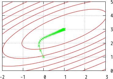
Run steepest descent method as follows:

# steepest_descent ~loops:100 ~eta:2. (dgauss a b) (gauss a b) [%vec [0.; 1.]];;
Loop 1: f x = -0.88288, x = -0.15576 1.46728
Loop 2: f x = -0.930997, x = -0.222322 1.80448
...
Loop 99: f x = -1, x = 0.999342 2.99959
Loop 100: f x = -1, x = 0.999392 2.99962
- : unit = ()

Our program successfully found the minimum point (exact solution = (1, 3)). You can control speed of convergence by changing a value of the learning rate.

Fig 2. Convergence of steepest descent (100 steps)

Bisection search of learning rate by Wolfe conditions

Sample program: examples/optimization/steepest_descent_wolfe.ml

Using too large learning rates may go through a minimal point (zigzag convergence), but quite small learning rates slowly reach a solution. In this section, we introduce an approach to find a learning rate achieving fast convergence: Wolfe conditions are used for finding an suitable learning rate. Wolfe conditions are

$f(\bm{x}+\alpha\bm{p})\le f(\bm{x})+c_1\alpha\bm{p}^\top\bm{\nabla}f(\bm{x})$, and
$\bm{p}^\top\bm{\nabla}f(\bm{x}+\alpha\bm{p})\ge c_2\bm{p}^\top\bm{\nabla}f(\bm{x})$

where $\bm{p}$ is a search direction, and $0<c_1<c_2<1$. These conditions give the upper bound and the lower bound of learning rate $\alpha$. We can find a learning rate satisfying the conditions by bisection search:

# let wolfe_search ?(c1=1e-4) ?(c2=0.9) ?(init=1.0) df f p x =
    let middle lo hi = 0.5 *. (lo +. hi) in
    let upper alpha = function (* Compute a new upper bound *)
      | None -> 2.0 *. alpha
      | Some hi -> middle alpha hi
    in
    let q = dot p (df x) in
    let y = f x in
    let xap = Vec.create (Vec.dim x) in
    let rec aux lo hi alpha =
      ignore (copy ~y:xap x); (* xap := x *)
      axpy ~alpha p xap; (* xap := xap + alpha * p *)
      if f xap > y +. c1 *. alpha *. q then aux lo (Some alpha) (middle lo alpha)
      else if dot p (df xap) < c2 *. q then aux alpha hi (upper alpha hi)
      else alpha (* Both of two conditions are satisfied. *)
    in
    aux 0.0 None init
  ;;
val wolfe_search :
  ?c1:float -> ?c2:float -> ?init:float ->
  (('a, 'b) vec -> ('a, 'c) vec) ->
  (('a, 'b) vec -> float) -> ('a, 'd) vec -> ('a, 'b) vec -> float = <fun>

wolfe_search ?c1 ?c2 ?init df f p x returns a learning rate satisfying Wolfe conditions. Optional argument init indicates the initial value of bisection search. If computation cost of a target function and its derivative is quite large, wolfe_search is inefficient.

The following code implements steepest descent method with automatic search of learning rates by Wolfe conditions:

# let steepest_descent_wolfe ~loops df f x =
    for i = 1 to loops do
      let p = Vec.neg (df x) in
      let eta = wolfe_search df f p x in (* Obtain a suitable learning rate *)
      axpy ~alpha:eta p x;
      printf "Loop %d: f x = %g, x = @[%a@]@." i (f x) pp_rfvec x
    done;;
val steepest_descent_wolfe :
  loops:int ->
  (('a, 'b) vec -> ('a, 'c) vec) ->
  (('a, 'b) vec -> float) -> ('a, 'b) vec -> unit = <fun>

steep_descent_wolfe achieves faster convergence as follows:

# steepest_descent_wolfe ~loops:60 (dgauss a b) (gauss a b) [%vec [0.; 1.]];;
Loop 1: f x = -0.83552, x = -0.0778801 1.23364
Loop 2: f x = -0.877268, x = -0.135404 1.43875
...
Loop 59: f x = -1, x = 0.999683 2.9998
Loop 60: f x = -1, x = 0.999731 2.99983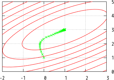

Fig 3. Convergence of steepest descent + Wolfe conditions (60 steps)

The convergence of Fig 3 is similar to that of Fig 2 (naive steepest descent described at the previous section), but the former is faster than the latter.

Newton method

Sample program: examples/optimization/newton.ml

Newton method (a.k.a., Newton-Raphson method) is also a kind of iterative approach using the second derivative of a target function addition to the first:

$\bm{x}^{(t+1)} = \bm{x}^{(t)} - \eta\Bigl(\bm{\nabla}^2 f(\bm{x}^{(t)})\Bigr)^{-1} \bm{\nabla} f(\bm{x}^{(t)}).$

The second derivative (often called Hessian matrix) is defined by

$\bm{\nabla}^2 f = \begin{pmatrix} \displaystyle\frac{\partial f}{\partial x_1\partial x_1}&\cdots& \displaystyle\frac{\partial f}{\partial x_1\partial x_n}\\ \vdots&\ddots&\vdots\\ \displaystyle\frac{\partial f}{\partial x_n\partial x_1}&\cdots& \displaystyle\frac{\partial f}{\partial x_n\partial x_n}\\ \end{pmatrix}.$

Newton method is implemented by using sytri and symv as follows:

# let newton ~loops ~eta ddf df f x =
    for i = 1 to loops do
      let h = ddf x in
      sytri h; (* h := h^(-1) *)
      ignore (symv ~alpha:(~-. eta) h (df x) ~beta:1. ~y:x); (* x := x - eta * h * (df x) *)
      printf "Loop %d: f = %g, x = @[%a@]@." i (f x) pp_rfvec x
    done;;
val newton :
  loops:int -> eta:float ->
  (('a, 'b) vec -> ('a, 'a, 'c) mat) ->
  (('a, 'b) vec -> ('a, 'd) vec) ->
  (('a, 'b) vec -> float) -> ('a, 'b) vec -> unit = <fun>

The Hessian matrix of the Gaussian function is given as

$\bm{\nabla}^2f(\bm{x})= -\exp\left(\frac{1}{2}(\bm{x}-\bm{b})^\top\bm{A}(\bm{x}-\bm{b})\right) \left(\bm{A}(\bm{x}-\bm{b})(\bm{x}-\bm{b})^\top\bm{A}^\top+\bm{A}\right).$

# let ddgauss a b x =
    let a' = Mat.copy a in
    ignore (syr (symv a (Vec.sub x b)) a'); (* a' := a' + a * (x-b) * (x-b)^T * a^T *)
    Mat.scal (gauss a b x) a';
    a';;
val ddgauss :
  ('a, 'a, 'b) mat -> ('a, 'c) vec -> ('a, 'd) vec -> ('a, 'a, 'e) mat =
  <fun>

where syr and Mat.scal are BLAS functions.

Try newton:

# newton ~loops:20 ~eta:0.4 (ddgauss a b) (dgauss a b) (gauss a b) [%vec [0.; 1.]];;
Loop 1: f = -0.99005, x = 0.8 2.6
Loop 2: f = -0.996503, x = 0.881633 2.76327
...
Loop 19: f = -1, x = 0.99998 2.99996
Loop 20: f = -1, x = 0.999988 2.99998
- : unit = ()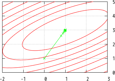

Fig 4. Convergence of Newton method (20 steps)

Newton method finds a minimal fast, while the approach has two problems:

Convergence of the iteration is not guaranteed if a Hessian matrix is not positive-definite symmetric. You need to give an initial point close to a minimal for finding the minimal because a Hessian matrix is positive-definite at points near a minimal. Newton method starting from an initial point far from a minimal fails. For example, function newton outputs a wrong result if you pass (0, -2) as an initial point since the Hessian matrix at (0, -2) is not positive-definite.
Computation of Hessian matrix and its inverse takes high cost. In addition, a target function is too complex to analytically compute its Hessian matrix in practical cases.

Quasi-Newton method

Sample program: examples/optimization/quasi_newton.ml

Quasi-Newton method is like Newton method, but an approximated inverse Hessian matrix is used. Several approximation approaches has been proposed, while we only introduce BFGS (Broyden-Fletcher-Goldfarb-Shanno) algorithm in this section.

Let $\bm{H}_t$ be an approximated inverse Hessian matrix at time step $t$, then the iteration of Quasi-Newton method is defined as

$\bm{x}_{t+1}=\bm{x}_t-\eta_t\bm{H}_t\bm{\nabla}\bm{f}(\bm{x}_t).$

The inverse Hessian approximated BFGS is computed by

$\bm{H}_{t+1}=\bm{H}_t +\left(1+\frac{\bm{y}_t^\top\bm{H}_t\bm{y}_t}{\bm{y}_t^\top\bm{s}_t}\right) \frac{\bm{s}_t\bm{s}_t^\top}{\bm{y}_t^\top\bm{s}_t} -\frac{\bm{H}_t\bm{y}_t\bm{s}_t^\top+\bm{s}_t\bm{y}_t^\top\bm{H}_t^\top}{\bm{y}_t^\top\bm{s}_t}$

where $\bm{s}_t=\bm{x}_{t+1}-\bm{x}_t$ and $\bm{y}_t=\bm{\nabla}\bm{f}(\bm{x}_{t+1})-\bm{\nabla}\bm{f}(\bm{x}_t)$. $\bm{H}_0$ is an identity matrix. A learning rate at each time step is chosen by Wolfe conditions for keeping $\bm{H}_t$ is positive-definite.

The following function update_h takes $\bm{H}_t$, $\bm{y}_t$ and $\bm{s}_t$, and destructively assigns $\bm{H}_{t+1}$ into the memory of argument $\bm{H}_t$ (parameter ?up specifies using upper or lower triangular of $\bm{H}_t$).

# let update_h ?up h y s =
    let rho = 1. /. dot y s in
    let hy = symv ?up h y in
    ignore (ger ~alpha:(~-. rho) hy s h); (* h := h - rho * hy * s^T *)
    ignore (ger ~alpha:(~-. rho) s hy h); (* h := h - rho * s * hy^T *)
    ignore (syr ?up ~alpha:((1. +. dot y hy *. rho) *. rho) s h)
  ;;
val update_h :
  ?up:bool -> ('a, 'a, 'b) mat -> ('a, 'c) vec -> ('a, 'd) vec -> unit = <fun>

Using update_h, Quasi-Newton method is implemented as follows:

# let quasi_newton ~loops df f x0 =
    let h = Mat.identity (Vec.dim x0) in (* an approximated inverse Hessian *)
    let rec aux i x df_dx =
      if i <= loops then begin
        let s = symv ~alpha:(-1.) h df_dx in (* search direction *)
        scal (wolfe_search df f s x) s;
        let x' = Vec.add x s in
        let df_dx' = df x' in
        let y = Vec.sub df_dx' df_dx in
        if dot y s > 1e-9 then begin (* Avoid divergence *)
          update_h h y s; (* Update an approximated inverse Hessian *)
          printf "Loop %d: f x = %g, x = @[%a@]@." i (f x) pp_rfvec x;
          aux (i + 1) x' df_dx'
        end
      end
    in
    aux 1 x0 (df x0)
  ;;
val quasi_newton :
  loops:int ->
  (('a, 'b) vec -> ('a, 'c) vec) ->
  (('a, 'b) vec -> float) -> ('a, 'b) vec -> unit = <fun>

Quasi-Newton method converges by iteration of only 7 steps:

# quasi_newton ~loops:10 (dgauss a b) (gauss a b) [%vec [0.0; 1.0]];;
Loop 1: f x = -0.83552, x = -0.0778801 1.23364
Loop 2: f x = -0.919791, x = -0.508032 2.76323
Loop 3: f x = -0.957169, x = -0.301939 2.23073
Loop 4: f x = -0.991233, x = 0.949811 3.27059
Loop 5: f x = -0.999928, x = 0.968443 3.00589
Loop 6: f x = -1, x = 1.00043 3
Loop 7: f x = -1, x = 0.999999 3
- : unit = ()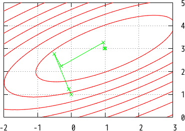

Fig 5. Convergence of Quasi-Newton method (7 steps)

The search direction at early steps of Quasi-Newton is wrong because $\bm{H}_t$ does not converge yet. However, after some steps, $\bm{H}_t$ approximates an inverse Hessian well, and convergence gets faster.

Visualization tips

Sample program: examples/optimization/visualization.ml

Figures in this article are plotted by gnuplot, an awesome graphing tool. In this section, we introduce how to draw figures like Fig 2, 3, 4, and 5 (i.e., visualization of convergence) by SLAP and gnuplot. SLAP provides no interface to gnuplot, but the visualization is not difficult.

Note: an OCaml library, Gnuplot-OCaml, is an interface to gnuplot from OCaml, while it does not support 3D graphs. Thus we don’t use this library in this section.

Using gnuplot from OCaml

Gnuplot is usually used on console (or called from a shell script):

$ gnuplot
gnuplot> plot sin(x)  # Plot a sine curve

The above command shows a figure of a sine curve on a window. You can use gnuplot from OCaml by using pipes:

# let gnuplot f =
    let oc = Unix.open_process_out "gnuplot" in (* Open a pipe to gnuplot *)
    let ppf = formatter_of_out_channel oc in (* For fprintf *)
    f ppf; (* Send gnuplot commands *)
    pp_print_flush ppf (); (* Flush an output buffer. *)
    print_endline "Press Enter to exit gnuplot";
    ignore (read_line ()); (* Prevent gnuplot from immediately exiting *)
    ignore (Unix.close_process_out oc) (* Exit gnuplot *)
  ;;
val gnuplot : (formatter -> unit) -> unit = <fun>

# gnuplot (fun ppf -> fprintf ppf "plot sin(x)\n");; (* Plot a sine curve *)

Note: if you pass command-line option -perisist to gnuplot (i.e., "gnuplot -persist" instead of "gnuplot") at the second line, a window is kept after gnuplot exited.

3D graph

plot command (in the previous section) plots 2D graphs, and splot command draws 3D graphs. The following example draws a 3D graph like Fig 1 (without contour):

# gnuplot (fun ppf ->
    fprintf ppf "set hidden3d\n\
                 set isosamples 30\n\
                 splot -exp((-0.1*(x-1)**2 - 0.2*(y-3)**2 + 0.2*(x-1)*(y-3)) / 2.0)\n");;

The drawn function -exp((-0.1*(x-1)**2 - 0.2*(y-3)**2 + 0.2*(x-1)*(y-3)) / 2.0) is the same as the target function in this article. However we want to directly plot function gauss (defined in OCaml) for simplicity and maintainability of code. The key idea to draw an OCaml function is to pass data points to splot command: splot can plot not only functions defined in gnuplot but also data points like:

gnuplot> splot '-' with lines  # Plot data points given from stdin
# x y z
  1 1 1
  1 2 2
  1 3 3

  2 1 2
  2 2 4
  2 3 6

  3 1 3
  3 2 6
  3 3 9

We can plot OCaml functions by conversion into data points:

# let splot_fun
      ?(option = "") ?(n = 10)
      ?(x1 = -10.0) ?(x2 = 10.0) ?(y1 = -10.0) ?(y2 = 10.0) ppf f =
    let cx = (x2 -. x1) /. float n in
    let cy = (y2 -. y1) /. float n in
    fprintf ppf "splot '-' %s@\n" option;
    for i = 0 to n do
      for j = 0 to n do
        let x = cx *. float i +. x1 in
        let y = cy *. float j +. y1 in
        let z = f [%vec [x; y]] in
        fprintf ppf "%g %g %g@\n" x y z;
      done;
      fprintf ppf "@\n"
    done;
    fprintf ppf "end@\n"
  ;;
val splot_fun :
  ?option:bytes ->
  ?n:int ->
  ?x1:float ->
  ?x2:float ->
  ?y1:float ->
  ?y2:float -> formatter -> ((Slap.Size.two, 'a) vec -> float) -> unit =
  <fun>

splot_fun ?option ?n ?x1 ?x2 ?y1 ?y2 ppf f draws the 3D graph of OCaml function f where

?option is a string of options for splot command,
?n is the number of points,
?x1 and ?x2 specify the range of x coordinates, and
?y1 and ?y2 specify the range of y coordinates.

Using splot, gauss can be plotted as follows:

# gnuplot (fun ppf ->
      fprintf ppf "set hidden3d\n";
      splot_fun ~option:"with lines" ~n:30 ppf (gauss a b));;

Plotting contour

You can plot contour by set contour command.

# gnuplot (fun ppf ->
      fprintf ppf "set contour             # Plot contour\n\
                   set view 0,0            # Fix a view\n\
                   unset surface           # Don't show a 3D surface\n\
                   set cntrparam levels 15 # Levels of contour\n";
      splot_fun ~option:"with lines" ~n:50 ppf (gauss a b));;

Plotting a line graph of convergence

Line graphs of convergence (like Fig 2, 3, 4, and 5) are 2D, but we draw them as 3D graphs because we will overlay a line graph on a contour graph.

# let steepest_descent ppf ~loops ~eta df f x =
    fprintf ppf "splot '-' with linespoints linetype 2 title ''@\n\
                 %a 0@\n" pp_rfvec x;
    for i = 1 to loops do
      axpy ~alpha:(~-. eta) (df x) x; (* x := x - eta * (df x) *)
      fprintf ppf "%a 0@\n" pp_rfvec x (* z coordinate = 0 *)
    done;
    fprintf ppf "end@\n"
  ;;
val steepest_descent :
  formatter ->
  loops:int ->
  eta:float -> (('a, 'b) vec -> ('a, 'c) vec) -> 'd -> ('a, 'b) vec -> unit =
  <fun>

# gnuplot (fun ppf ->
      fprintf ppf "set view 0,0 # Fix a view@\n\
                   set xrange [-2:3]@\n\
                   set yrange [0:5]@\n";
      steepest_descent ppf
        ~loops:100 ~eta:2.0 (dgauss a b) (gauss a b) [%vec [0.0; 1.0]]);;

Overlaying a line graph on a contour graph

Overlaying two graphs is achieved by set multiplot. The following code displays a graph similar to Fig 2, while we used additional a few commands for improvement of visualization. Sample program examples/optimization/visualization.ml contains the commands, and shows the same graph as Fig 2.

# gnuplot (fun ppf ->
      fprintf ppf "set multiplot\n\
                   set view 0,0 # Fix a view\n\
                   set xrange [-2:3]@\n\
                   set yrange [0:5]@\n";
      steepest_descent ppf
        ~loops:100 ~eta:2.0 (dgauss a b) (gauss a b) [%vec [0.0; 1.0]];
      fprintf ppf "set contour             # Plot contour\n\
                   unset surface           # Don't show a 3D surface\n\
                   set cntrparam levels 15 # Levels of contour\n";
      splot_fun ~option:"with lines" ~n:50 ppf (gauss a b));;